使用GAN生成MNIST数据集(Pytorch)

前言

在上一篇文章里实现了MNIST手写数据集的识别之后,趁热打铁,这一篇文章使用GAN来实现MNIST数据集的生成。2014年Ian Goodfellow的那篇GAN是我接触的第一篇有关机器学习的文章。那篇文章被称为GAN的开山之作,它提出了一种新的生成式框架,其中包括生成模型和鉴别模型。生成模型用于描述数据的分布,生成尽可能拟合真实数据的分布,而鉴别模型用于对生成模型各个迭代轮次产生的结果进行评估,其中利用到了一种博弈的思想。

1

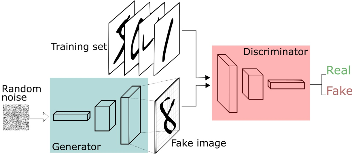
在GAN模型的后面是大量的度量单位和公式推导,在这里我们不做详细说明。今天主要是通过GAN的方式利用两个模型(卷积网络和线性网络)实现MNIST数据集的生成。

线性模型

首先还是模块的导入,对应相关模块的功能在上一篇文章已做了相关说明。

1
2
3
4
5
6
7
import torch
import torchvision
import torch.nn as nn
from torchvision import datasets,transforms
from torchvision.utils import save_image
from torch.autograd import Variable
from torch.utils.data import DataLoader

参数定义,其中z_dimension是随机生成噪声的维度,这里定义为100维,可以自定义。

1
2
3
4
5
6
7
batch_size = 64
epochs = 3
z_dimension = 100
transforms = transforms.Compose([
transforms.ToTensor(),
transforms.Normalize((0.1307,),(0.3081,))
])

数据集的加载,由于是生成MNIST数据集,所以这次不需要对测试集进行加载,通过训练集进行训练生成即可。

1
2
train_set = datasets.MNIST("data",train=True,transform=transforms,download=True)
train_loader = DataLoader(train_set,batch_size=batch_size,shuffle=True)

判别器的定义,采用三层的线性模型。Linear的两个参数分别是输出层和隐藏层。在第一层的输出层是784是因为MNIST图片大小是1*28*28,中间的隐藏层可以自定义,线性变换之后采用一个LeakyReLU的激活函数实现非线性映射,参数0.2是激活函数的斜率。最后使用Sigmoid函数实现概率值的映射,sigmoid常用作二分类问题。在这里使用sigmoid函数得到一个0到1的概率进行二分类。在forward函数中还采用了一个squeeze函数,这个函数主要对数据的维度进行压缩,去掉维数为1的的维度,默认是将a中所有为1的维度删掉。x.squeeze(-1)用于将二维压缩为一维。

1
2
3
4
5
6
7
8
9
10
11
12
13
14
15
16
class Discriminator(nn.Module):
def __init__(self):
super(Discriminator, self).__init__()
self.dis = nn.Sequential(
nn.Linear(784,256),
nn.LeakyReLU(0.2),
nn.Linear(256,256),
nn.LeakyReLU(0.2),
nn.Linear(256,1),
nn.Sigmoid()
)

def forward(self,x):
x = self.dis(x)
x = x.squeeze(-1)
return x

生成器的定义,生成器和判别器的定义相同,也是经过一个三层的线性模型,其中第一个Linear函数的第一个参数是100,这是在前面参数定义的z_dimension = 100也就是随机噪声的维度,在生成器中使用的激活函数是Relu激活函数,最后一层Linear函数的输出层是784维对应了MNIST数据的大小,之后使用Tanh激活函数是希望生成的假的图片数据分布能够在-1~1之间。

1
2
3
4
5
6
7
8
9
10
11
12
13
14
15
class Generator(nn.Module):
def __init__(self):
super(Generator, self).__init__()
self.gen = nn.Sequential(
nn.Linear(100,256),
nn.ReLU(True),
nn.Linear(256,256),
nn.ReLU(True),
nn.Linear(256,784),
nn.Tanh()
)
def forward(self,x):
x = self.gen(x)
x = x.squeeze(-1)
return x

实例化生成器模型和判别器模型。

1
2
Dis = Discriminator()
Gen = Generator()

定义损失函数和优化器,其中BCELoss是单目标二分类交叉熵函数。

1
2
3
criterion = nn.BCELoss()
Dis_optimizer = torch.optim.Adam(Dis.parameters(),lr=0.0003)
Gen_optimizer = torch.optim.Adam(Gen.parameters(),lr=0.0003)

开始训练。训练集中包含图片和标签数据。通过img.size(0)可以得到每一批数据的数量,也就是我们之前设定的batch_size大小,随后通过view函数将数据进行拉平成二维方便后续的处理,之后分别计算真实图片和假图片的损失并进行迭代训练,最后将生成的真实图片和假的图片保存在img文件夹下。

1
2
3
4
5
6
7
8
9
10
11
12
13
14
15
16
17
18
19
20
21
22
23
24
25
26
27
28
29
30
31
32
33
34
35
36
37
38
39
40
41
42
43
44
for epoch in range(epochs):
for batch_idx, (img,target) in enumerate(train_loader):
num_img = img.size(0)
#训练判别器
img = img.view(num_img,-1) #拉成64*784
real_img = Variable(img) #将tensor变成Variable计算
real_label = Variable(torch.ones(num_img)) #真图片label为1
fake_label = Variable(torch.zeros(num_img)) #假图片label为0

#计算真实图片的loss
real_out = Dis(real_img) #图片放入判别器
d_loss_real = criterion(real_out,real_label) #计算loss
real_scores = real_out

#计算假图片的loss
z = Variable(torch.randn(num_img,z_dimension)) #随机生成一些噪声
fake_img = Gen(z)
fake_out = Dis(fake_img)
d_loss_fake = criterion(fake_out,fake_label)
fake_scores = fake_out

d_loss = d_loss_real + d_loss_fake
Dis_optimizer.zero_grad()
d_loss.backward()
Dis_optimizer.step()

#训练生成器
z = Variable(torch.randn(num_img, z_dimension)) # 随机生成一些噪声
fake_img = Gen(z)
output = Dis(fake_img)
g_loss = criterion(output,real_label)

Gen_optimizer.zero_grad()
g_loss.backward()
Gen_optimizer.step()

if batch_idx % 100 ==0:
print('Epoch {},d_loss: {:.6f},g_loss: {:.6f},D real: {:.6f},D fake: {:.6f}'.format( epoch,d_loss.item(),g_loss.item(),real_scores.data.mean(),fake_scores.data.mean()
))
if epoch == 0:
real_images = to_img(real_img.data)
save_image(real_images.data,'img/real_images.png')
fake_images = to_img(fake_img.data)
save_image(fake_images.data,"img/fake_images-{}.png".format(epoch))

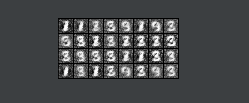
结果展示,下图是训练3轮次后生成的图像。因为代码是在自己电脑上跑的所以训练的次数比较少,生成的图片不太清晰。
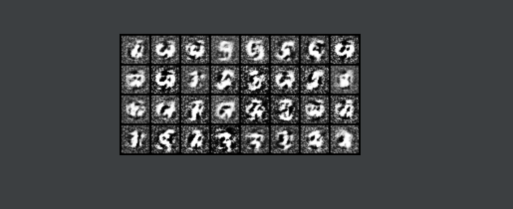
2

训练20轮次的结果

3

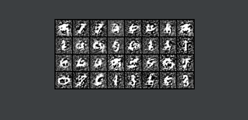
训练50轮次的结果,怎么感觉越训练越差了。。。后面再看看具体调优的事。

4

卷积模型

卷积模型和线性模型的代码主要是模型的定义处不太相同。

首先是判别器的定义,其中判别器采用的是两层的卷积模型和一层的全连接层

1
2
3
4
5
6
7
8
9
10
11
12
13
14
15
16
17
18
19
20
21
22
23
24
25
26
class Discriminator(nn.Module):
def __init__(self):
super(Discriminator, self).__init__()
self.conv1 = nn.Sequential(
nn.Conv2d(1,32,5,padding=2),#32,28,28
nn.LeakyReLU(0.2),
nn.MaxPool2d(2, stride=2),#32,14,14
)
self.conv2 = nn.Sequential(
nn.Conv2d(32, 64, 5, padding=2), #64,14,14
nn.LeakyReLU(0.2),
nn.MaxPool2d(2, stride=2), #64,7,7
)
self.fc = nn.Sequential(
nn.Linear(64*7*7,1024),
nn.LeakyReLU(0.2),
nn.Linear(1024,1),
nn.Sigmoid()
)
def forward(self,x):
x = self.conv1(x)
x = self.conv2(x)
x = x.view(x.size(0), -1) #将4维转为2维
x = self.fc(x)
x = x.squeeze(-1) #将2维转为1维
return x

其次是生成器的定义,生成器首先是经过一个全连接层,其中input_size是100也就是随机噪声的维度,num_feature是我们定义的数值为3136,这个可以自定义,只要最后转为[batch,1,28,28]形式就行。其中 BatchNorm2d函数用来做归一化处理,这里我们只写入了BatchNorm2d的第一个参数,也就是输入图像的通道数,所以刚开始是1。后面的通道数随着卷积操作的改变而改变。

1
2
3
4
5
6
7
8
9
10
11
12
13
14
15
16
17
18
19
20
21
22
23
24
25
26
27
28
29
30
31
class Generator(nn.Module):
def __init__(self, input_size, num_feature):
super(Generator, self).__init__()
self.fc = nn.Linear(input_size, num_feature) # batch, 3136=1x56x56
self.br = nn.Sequential(
nn.BatchNorm2d(1),
nn.ReLU(True)
)
self.downsample1 = nn.Sequential(
nn.Conv2d(1, 50, 3, stride=1,padding=1), # batch, 50, 56, 56
nn.BatchNorm2d(50),
nn.ReLU(True)
)
self.downsample2 = nn.Sequential(
nn.Conv2d(50, 25, 3, stride=1, padding=1), # batch, 25, 56, 56
nn.BatchNorm2d(25),
nn.ReLU(True)
)
self.downsample3 = nn.Sequential(
nn.Conv2d(25, 1, 2, stride=2), # batch, 1, 28, 28
nn.Tanh()
)

def forward(self, x):
x = self.fc(x)
x = x.view(x.size(0), 1, 56, 56)
x = self.br(x)
x = self.downsample1(x)
x = self.downsample2(x)
x = self.downsample3(x)
return x

实例化生成器和判别器

1
2
Dis = Discriminator()
Gen = Generator(z_dimension,3136)

进行训练,这里需要注意的是在训练的时候不需要使用view函数将img转为二维,这里直接对四维数据进行处理。剩下的操作和线性模型相同。

1
2
3
4
5
6
7
for epoch in range(epochs):
for batch_idx, (img,target) in enumerate(train_loader):
#训练判别器
# img = img.view(num_img,-1) #拉成64*784
real_img = Variable(img) #将tensor变成Variable计算
real_label = Variable(torch.ones(num_img)) #真图片label为1
fake_label = Variable(torch.zeros(num_img)) #假图片label为0

线性模型完整代码

注意要在同级目录下创建一个img的文件夹

1
2
3
4
5
6
7
8
9
10
11
12
13
14
15
16
17
18
19
20
21
22
23
24
25
26
27
28
29
30
31
32
33
34
35
36
37
38
39
40
41
42
43
44
45
46
47
48
49
50
51
52
53
54
55
56
57
58
59
60
61
62
63
64
65
66
67
68
69
70
71
72
73
74
75
76
77
78
79
80
81
82
83
84
85
86
87
88
89
90
91
92
93
94
95
96
97
98
99
100
101
102
103
104
105
106
107
108
109
110
111
112
113
import torch
import torchvision
import torch.nn as nn
from torchvision import datasets,transforms
from torchvision.utils import save_image
from torch.autograd import Variable
from torch.utils.data import DataLoader

#用来还原真实数据
def to_img(x):
out = 0.5 * (x + 1)
out = out.clamp(0,1) #将随机变化的数值限制在一个给定的区间
out = out.view(-1,1,28,28)
return out

batch_size = 64
epochs = 50
z_dimension = 100

transforms = transforms.Compose([
transforms.ToTensor(),
transforms.Normalize((0.1307,),(0.3081,))
])

train_set = datasets.MNIST("data",train=True,transform=transforms,download=True)
train_loader = DataLoader(train_set,batch_size=batch_size,shuffle=True)

class Discriminator(nn.Module):
def __init__(self):
super(Discriminator, self).__init__()
self.dis = nn.Sequential(
nn.Linear(784,256),
nn.LeakyReLU(0.2),
nn.Linear(256,256),
nn.LeakyReLU(0.2),
nn.Linear(256,1),
nn.Sigmoid()
)

def forward(self,x):
x = self.dis(x)
x = x.squeeze(1)
return x

class Generator(nn.Module):
def __init__(self):
super(Generator, self).__init__()
self.gen = nn.Sequential(
nn.Linear(100,256), #输入一个100维的0~1之间的高斯分布
nn.ReLU(True),
nn.Linear(256,256),
nn.ReLU(True),
nn.Linear(256,784),
nn.Tanh()
)
def forward(self,x):
x = self.gen(x)
x = x.squeeze(-1)
return x

Dis = Discriminator()
Gen = Generator()

criterion = nn.BCELoss()
Dis_optimizer = torch.optim.Adam(Dis.parameters(),lr=0.0003)
Gen_optimizer = torch.optim.Adam(Gen.parameters(),lr=0.0003)

for epoch in range(epochs):
for batch_idx, (img,_) in enumerate(train_loader):
num_img = img.size(0) #获取图片大小 64
#训练判别器
img = img.view(num_img,-1) #拉平成64*784
real_img = Variable(img) #将tensor变成Variable计算
real_label = Variable(torch.ones(num_img)) #真图片label为1
fake_label = Variable(torch.zeros(num_img)) #假图片label为0

#计算真实图片的loss
real_out = Dis(real_img) #图片放入判别器
d_loss_real = criterion(real_out,real_label) #计算loss
real_scores = real_out

#计算假图片的loss
z = Variable(torch.randn(num_img,z_dimension)) #随机生成一些噪声
fake_img = Gen(z)
fake_out = Dis(fake_img)
d_loss_fake = criterion(fake_out,fake_label)
fake_scores = fake_out

d_loss = d_loss_real + d_loss_fake
Dis_optimizer.zero_grad()
d_loss.backward()
Dis_optimizer.step()


#训练生成器
z = Variable(torch.randn(num_img, z_dimension)) # 随机生成一些噪声
fake_img = Gen(z)
output = Dis(fake_img)
g_loss = criterion(output,real_label)

Gen_optimizer.zero_grad()
g_loss.backward()
Gen_optimizer.step()

if batch_idx % 100 ==0:
print('Epoch {},d_loss: {:.6f},g_loss: {:.6f},D real: {:.6f},D fake: {:.6f}'.format(
epoch,d_loss.item(),g_loss.item(),real_scores.data.mean(),fake_scores.data.mean()
))
if epoch == 0:
real_images = to_img(real_img.data)
save_image(real_images.data,'img/real_images.png')
fake_images = to_img(fake_img.data)
save_image(fake_images.data,"img/fake_images-{}.png".format(epoch))

卷积模型完整代码

1
2
3
4
5
6
7
8
9
10
11
12
13
14
15
16
17
18
19
20
21
22
23
24
25
26
27
28
29
30
31
32
33
34
35
36
37
38
39
40
41
42
43
44
45
46
47
48
49
50
51
52
53
54
55
56
57
58
59
60
61
62
63
64
65
66
67
68
69
70
71
72
73
74
75
76
77
78
79
80
81
82
83
84
85
86
87
88
89
90
91
92
93
94
95
96
97
98
99
100
101
102
103
104
105
106
107
108
109
110
111
112
113
114
115
116
117
118
119
120
121
122
123
124
125
126
127
128
129
130
131
132
133
134
135
136
137
138
139
140
import torch
import torchvision
import torch.nn as nn
from torchvision import datasets,transforms
from torchvision.utils import save_image
from torch.autograd import Variable
from torch.utils.data import DataLoader

#还原真实数据
def to_img(x):
out = 0.5 * (x + 1)
out = out.clamp(0,1) #将随机变化的数值限制在一个给定的区间
out = out.view(-1,1,28,28)
return out

batch_size = 16
epochs = 3
z_dimension = 100

transforms = transforms.Compose([
transforms.ToTensor(),
transforms.Normalize((0.1307,),(0.3081,))
])

train_set = datasets.MNIST("data",train=True,transform=transforms,download=True)
train_loader = DataLoader(train_set,batch_size=batch_size,shuffle=True)

class Discriminator(nn.Module):
def __init__(self):
super(Discriminator, self).__init__()
self.conv1 = nn.Sequential(
nn.Conv2d(1,32,5,padding=2),#32,28,28
nn.LeakyReLU(0.2),
nn.MaxPool2d(2, stride=2),#32,14,14
)
self.conv2 = nn.Sequential(
nn.Conv2d(32, 64, 5, padding=2), #64,14,41
nn.LeakyReLU(0.2),
nn.MaxPool2d(2, stride=2), #64,7,7
)
self.fc = nn.Sequential(
nn.Linear(64*7*7,1024),
nn.LeakyReLU(0.2),
nn.Linear(1024,1),
nn.Sigmoid()
)


def forward(self,x):
x = self.conv1(x)
x = self.conv2(x)
x = x.view(x.size(0), -1)
x = self.fc(x)
x = x.squeeze(-1)
return x

class Generator(nn.Module):
def __init__(self, input_size, num_feature):
super(Generator, self).__init__()
self.fc = nn.Linear(input_size, num_feature) # batch, 3136=1x56x56
self.br = nn.Sequential(
nn.BatchNorm2d(1),
nn.ReLU(True)
)
self.downsample1 = nn.Sequential(
nn.Conv2d(1, 50, 3, stride=1,padding=1), # batch, 50, 56, 56
nn.BatchNorm2d(50),
nn.ReLU(True)
)
self.downsample2 = nn.Sequential(
nn.Conv2d(50, 25, 3, stride=1, padding=1), # batch, 25, 56, 56
nn.BatchNorm2d(25),
nn.ReLU(True)
)
self.downsample3 = nn.Sequential(
nn.Conv2d(25, 1, 2, stride=2), # batch, 1, 28, 28
nn.Tanh()
)

def forward(self, x):
x = self.fc(x)
x = x.view(x.size(0), 1, 56, 56)
x = self.br(x)
x = self.downsample1(x)
x = self.downsample2(x)
x = self.downsample3(x)
return x


Dis = Discriminator()
Gen = Generator(z_dimension,3136)

criterion = nn.BCELoss()
Dis_optimizer = torch.optim.Adam(Dis.parameters(),lr=0.0003)
Gen_optimizer = torch.optim.Adam(Gen.parameters(),lr=0.0003)

for epoch in range(epochs):
for batch_idx, (img,_) in enumerate(train_loader):
#训练判别器
real_img = Variable(img) #将tensor变成Variable计算
real_label = Variable(torch.ones(num_img)) #真图片label为1
fake_label = Variable(torch.zeros(num_img)) #假图片label为0

#计算真实图片的loss
real_out = Dis(real_img) #图片放入判别器
d_loss_real = criterion(real_out,real_label) #计算loss
real_scores = real_out

#计算假图片的loss
z = Variable(torch.randn(num_img,z_dimension)) #随机生成一些噪声
fake_img = Gen(z)
fake_out = Dis(fake_img)
d_loss_fake = criterion(fake_out,fake_label)
fake_scores = fake_out

d_loss = d_loss_real + d_loss_fake
Dis_optimizer.zero_grad()
d_loss.backward()
Dis_optimizer.step()


#训练生成器
z = Variable(torch.randn(num_img, z_dimension)) # 随机生成一些噪声
fake_img = Gen(z)
output = Dis(fake_img)
g_loss = criterion(output,real_label)

Gen_optimizer.zero_grad()
g_loss.backward()
Gen_optimizer.step()

if batch_idx % 100 ==0:
print('Epoch {},d_loss: {:.6f},g_loss: {:.6f},D real: {:.6f},D fake: {:.6f}'.format(
epoch,d_loss.item(),g_loss.item(),real_scores.data.mean(),fake_scores.data.mean()
))
if epoch == 0:
real_images = to_img(real_img.data)
save_image(real_images.data,'img/real_images.png')
fake_images = to_img(fake_img.data)
save_image(fake_images.data,"img/fake_images-{}.png".format(epoch))