前言
FGSM的全称是Fast Gradient Sign Method(快速梯度下降法),在白盒环境下,通过求出模型对输入的导数,然后用符号函数得到其具体的梯度方向,接着乘以一个步长,得到的“扰动”加在原来的输入 上就得到了在FGSM攻击下的样本。本文将实现在Pytorch框架下使用FGSM攻击MNIST数据集
训练模型的保存
通过之前MNIST识别的代码实现,我们就可以实现模型的保存。只需要在最后加上一行代码即可。
1 | torch.save(model.state_dict(), "mnist_model.pth") |
save函数有两个参数,第一个参数是模型的状态。其中model.state_dict()只保存模型权重参数,不保存模型结构,而model则保存整个模型的状态。这里我们使用model.state_dict(),第二个参数是路径和保存的文件名。这里我们保存在同级目录下,文件名是mnist_model.pth
训练模型完整代码如下:
1 | import torch |
攻击代码
相关模块的导入
1 | import torch |
可能遇到的错误
1 | OMP: Error #15: Initializing libomp.dylib, but found libiomp5.dylib already initialized. |
解决方法
1 | import os |
参数定义
其中epsilons是FGSM攻击所加的扰动,值不超过1。pretrained_model是预训练模型,也就是我们上面保存的训练模型。
1 | epsilons = [0, .05, .1, .15, .2, .25, .3] |
定义受攻击的模型
这里的模型与我们上面MNIST识别所定义的模型相同。我们使用两个卷积层和两个全连接层,具体定义如下:
1 | class Net(nn.Module): |
加载测试集
1 | test_loader = DataLoader( |
实例化模型
1 | model = Net() |
加载预训练模型
1 | model.load_state_dict(torch.load(pretrained_model)) |
定义模型的评估模式
这里设置eval进行训练默认不开启Dropout和BatchNormalization
1 | model.eval() |
定义FGSM攻击模型
在FGSM攻击模型函数中一共有3个参数,第一个参数是原始图片,第二个参数是攻击的扰动量,一般在0~1之间,第三个参数是图像关于求导之后的损失。最后由于对抗样本可能会在(0,1)范围之外,所以通过clamp函数将加扰动之后的图片限制在(0,1)之间。
1 | def fgsm_attack(image, epsilon, data_grad): |
定义测试函数
1 | def test( model, test_loader, epsilon ): |
开始训练
1 | accuracies = [] #记录准确率 |
训练结果
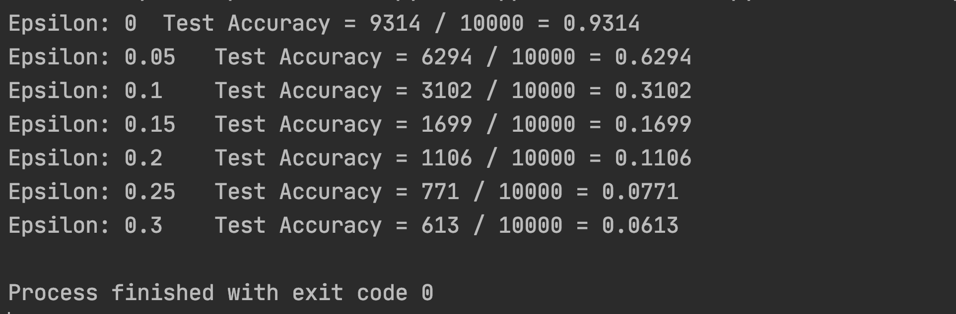
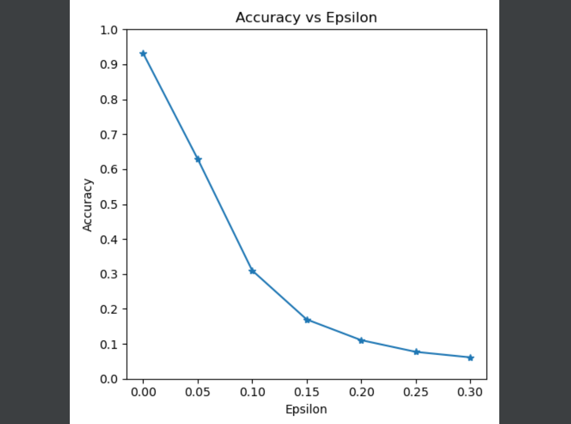
画出随着扰动值变化的准确率图
1 | plt.figure(figsize=(5,5)) |
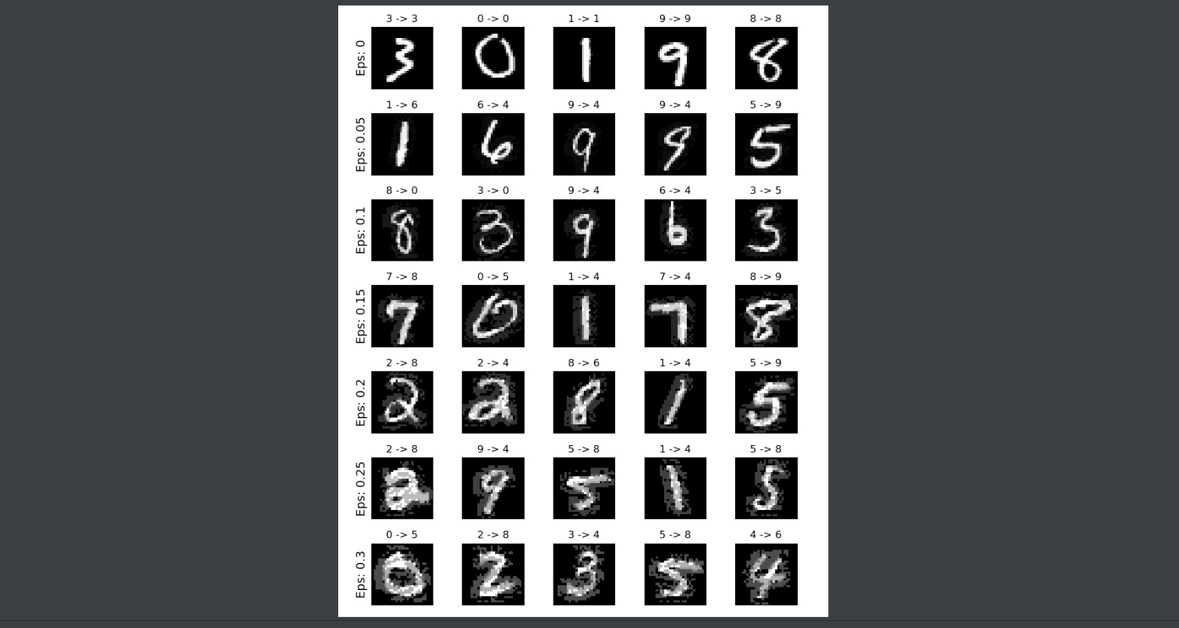
画出在不同扰动值下对抗实例图,每个扰动值对应5张照片。
1 | cnt = 0 |
FGSM攻击MNIST完整代码
1 | import torch |